Tutorial

These are examples of some basic scans that the user might perform on the high level interface. The examples have run on a virtual instrument defined in a later section. This documentation also serves as a testing basis to ensure that this the code always matches the functionality declared here.

Plot Motor Scan

Our first, simplest example is the user plotting a scan of the detector intensity as the motor moves from 0 to 2 exclusively in steps of 0.6.

>>> from Scans import *
>>> scan(theta, 0, 2, 0.6, 50)
Taking a count at theta=0.00 and two theta=0.00
Taking a count at theta=0.60 and two theta=0.00
Taking a count at theta=1.20 and two theta=0.00
Taking a count at theta=1.80 and two theta=0.00

The above is the simplest possible kind of default scan. The first parameter is the starting point, the second is the stopping point, the third is the step size, and the final parameter is the number of frames to measure at each point. For most cases, it should be sufficient, but there are many more options that can be layered on top.

>>> scan(theta, 0, 2, stride=0.6, frames=10)
Taking a count at theta=0.00 and two theta=0.00
Taking a count at theta=0.50 and two theta=0.00
Taking a count at theta=1.00 and two theta=0.00
Taking a count at theta=1.50 and two theta=0.00
Taking a count at theta=2.00 and two theta=0.00

Above, we’ve not used the default step parameter, but did use the stride parameter instead. Setting the stride instead of setting the step allow the instrument to slightly adjust the step size to ensure that the end point is included in the scan. In this example, the step size was decrease from 0.6 mm to 0.5 mm.

Note

Since we skipped the step parameter, we had to give the frames parameter by name.

The results of all scans are saved to a log file. The location of the log is set by the instrument scientist. The data from the scan above can be seen below.

mock_scan_02.dat

0.0	0.021182739966945238
0.5	1.359946067403626
1.0	1.5621816664312744
1.5	1.3559685463898044
2.0	0.8738762002145183

>>> s = scan(theta, 0, 2, 0.6, seconds=1, save="plot_example.png")
Taking a count at theta=0.00 and two theta=0.00
Taking a count at theta=0.60 and two theta=0.00
Taking a count at theta=1.20 and two theta=0.00
Taking a count at theta=1.80 and two theta=0.00

The save argument allows the figure to be saved to a file. Otherwise, the screen will show the plot interactively. Also, notice we’ve given the time for each measuremnt in seconds instead of frames. The values or minutes, hours, and uamps are also accepted.

There are many possibilities beyond the start, stop, step, and stride that have been introduced thus far. For example, count and gaps allow the user to specify the number of measurements and the number of gaps, respectively.

>>> scan(theta, start=0, stop=2, count=4, frames=5)
Taking a count at theta=0.00 and two theta=0.00
Taking a count at theta=0.67 and two theta=0.00
Taking a count at theta=1.33 and two theta=0.00
Taking a count at theta=2.00 and two theta=0.00
>>> scan(theta, start=0, stop=2, gaps=4, frames=5)
Taking a count at theta=0.00 and two theta=0.00
Taking a count at theta=0.50 and two theta=0.00
Taking a count at theta=1.00 and two theta=0.00
Taking a count at theta=1.50 and two theta=0.00
Taking a count at theta=2.00 and two theta=0.00

The user also has the option of fixing the steps size and number of measurements or gaps while leaving the ending position open.

>>> scan(theta, start=0, step=0.6, count=5, frames=5)
Taking a count at theta=0.00 and two theta=0.00
Taking a count at theta=0.60 and two theta=0.00
Taking a count at theta=1.20 and two theta=0.00
Taking a count at theta=1.80 and two theta=0.00
Taking a count at theta=2.40 and two theta=0.00
>>> scan(theta, start=0, stride=0.6, gaps=5, frames=5)
Taking a count at theta=0.00 and two theta=0.00
Taking a count at theta=0.60 and two theta=0.00
Taking a count at theta=1.20 and two theta=0.00
Taking a count at theta=1.80 and two theta=0.00
Taking a count at theta=2.40 and two theta=0.00
Taking a count at theta=3.00 and two theta=0.00

For when relative scans make more sense, it’s possible to request them by replacing start and stop with before and after.

>>> scan(theta, before=-1, after=1, stride=0.6, frames=5)
Taking a count at theta=2.00 and two theta=0.00
Taking a count at theta=2.50 and two theta=0.00
Taking a count at theta=3.00 and two theta=0.00
Taking a count at theta=3.50 and two theta=0.00
Taking a count at theta=4.00 and two theta=0.00

Since relative scans are fairly common, there’s a built in Scans.Spec.rscan() method which defaults to a relative scan, instead of an absolute.

>>> rscan(theta, -1, 1, 0.5, 5)
Taking a count at theta=3.00 and two theta=0.00
Taking a count at theta=3.50 and two theta=0.00
Taking a count at theta=4.00 and two theta=0.00
Taking a count at theta=4.50 and two theta=0.00
>>> theta
Theta is at 4.0

Note

Some combinations of values do not provide enough information to create a scan. A RuntimeError will be thrown if a scan cannot be constructed

>>> scan(theta, start=0, stop=0.6, after=2)
Traceback (most recent call last):
...
RuntimeError: Unable to build a scan with that set of options.

Motor Objects

We’ve been using the motor object theta, but we haven’t discussed how it works.

>>> theta()
4.0

Calling the object with no parameters returns the current position. This position can be changed by giving a new value in the function

>>> THETA()
4.0
>>> Theta()
4.0

The axis can be called by its name in lower case, in upper case, or as case in the IBEX block.

>>> theta(3.0)
>>> theta
Theta is at 3.0

We can also perform some relative changes with Python’s in place operators.

>>> theta += 1.5
>>> theta
Theta is at 4.5
>>> theta -= 4
>>> theta *= 2
>>> theta
Theta is at 1.0

Soft limits can be placed on motors with the low and high properties. Scans that attempt to exceed these values will throw an error.

>>> theta.low = 0
>>> theta.high = 2
>>> scan(theta, start=0, stop=10, count=21)
Traceback (most recent call last):
    ...
RuntimeError: Position 2.5 is above upper limit 2 of motor Theta
>>> theta.high = None

If there is no Motion object for a specific axis, the user can give the name in a string and use that. If the axis isn’t a string or a Motion object, the scan will fail. Also, the string must be the same case as in the IBEX block.

>>> scan("Theta", start=0, stop=10, stride=2, frames=5)
Taking a count at theta=0.00 and two theta=0.00
Taking a count at theta=2.00 and two theta=0.00
Taking a count at theta=4.00 and two theta=0.00
Taking a count at theta=6.00 and two theta=0.00
Taking a count at theta=8.00 and two theta=0.00
Taking a count at theta=10.00 and two theta=0.00
>>> scan("theta", start=0, stop=10, stride=2, frames=5)
Traceback (most recent call last):
    ...
RuntimeError: Unknown block theta.  Does the capitalisation match IBEX?
>>> scan(True, start=0, stop=10, count=5) # doctest: +NORMALIZE_WHITESPACE
Traceback (most recent call last):
    ...
TypeError: Cannot run scan on axis True. Try a string or a motion
object instead.  It's also possible that you may need to rerun
populate() to recreate your motion axes.

Perform Fits

Performing a fit on a measurement is merely a modification of performing the plot

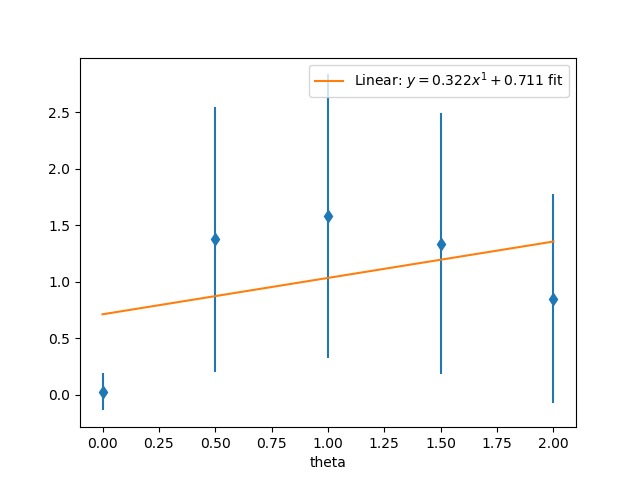
>>> fit = scan(theta, start=0, stop=2, stride=0.6, fit=Linear, frames=5)
Taking a count at theta=0.00 and two theta=0.00
Taking a count at theta=0.50 and two theta=0.00
Taking a count at theta=1.00 and two theta=0.00
Taking a count at theta=1.50 and two theta=0.00
Taking a count at theta=2.00 and two theta=0.00
>>> abs(fit["slope"] - 0.33) < 0.02
True

In this instance, the user requested a linear fit. The result was an array with the slope and intercept. The fit is also plotted over the original graph when finished.

>>> fit = scan(theta, start=0, stop=2, stride=0.6, fit=PolyFit(3), frames=5)
Taking a count at theta=0.00 and two theta=0.00
Taking a count at theta=0.50 and two theta=0.00
Taking a count at theta=1.00 and two theta=0.00
Taking a count at theta=1.50 and two theta=0.00
Taking a count at theta=2.00 and two theta=0.00
>>> abs(fit["x^0"]) < 0.1
True

Higher order polynomials are also supported

We can also plot the same scan against a Gaussian

>>> fit = scan(theta, start=0, stop=2, count=11, fit=Gaussian, frames=5, save="gaussian.png")
Taking a count at theta=0.00 and two theta=0.00
Taking a count at theta=0.20 and two theta=0.00
Taking a count at theta=0.40 and two theta=0.00
Taking a count at theta=0.60 and two theta=0.00
Taking a count at theta=0.80 and two theta=0.00
Taking a count at theta=1.00 and two theta=0.00
Taking a count at theta=1.20 and two theta=0.00
Taking a count at theta=1.40 and two theta=0.00
Taking a count at theta=1.60 and two theta=0.00
Taking a count at theta=1.80 and two theta=0.00
Taking a count at theta=2.00 and two theta=0.00
>>> abs(fit["center"] - 1.0) < 0.2
True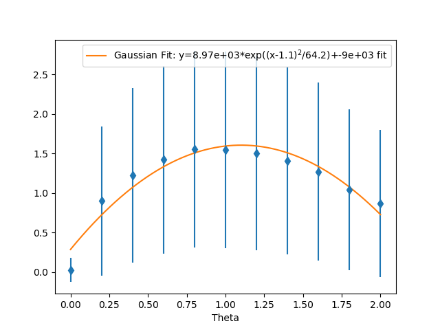

There is a simple peak finder as well. It finds the largest data point and then fits the local neighbourhood of points to a parabola to refine that point. The width of that neighbourhood is the parameter to PeakFit.

>>> fit = scan(theta, start=0, stop=2, count=11, fit=PeakFit(0.7), frames=5, save="peak.png")
Taking a count at theta=0.00 and two theta=0.00
Taking a count at theta=0.20 and two theta=0.00
Taking a count at theta=0.40 and two theta=0.00
Taking a count at theta=0.60 and two theta=0.00
Taking a count at theta=0.80 and two theta=0.00
Taking a count at theta=1.00 and two theta=0.00
Taking a count at theta=1.20 and two theta=0.00
Taking a count at theta=1.40 and two theta=0.00
Taking a count at theta=1.60 and two theta=0.00
Taking a count at theta=1.80 and two theta=0.00
Taking a count at theta=2.00 and two theta=0.00
>>> abs(fit["peak"] - 1.0) < 0.1
True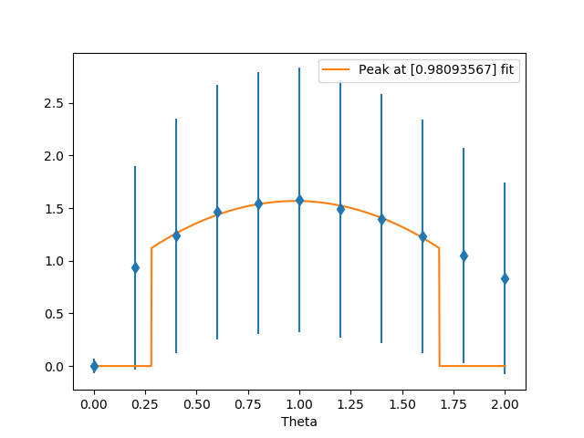

There is a similar fit model for the error function, which helps to approximate an edge.

>>> fit = scan(theta, start=1, stop=3, count=11, fit=Erf, frames=5, save="erf.png")
Taking a count at theta=1.00 and two theta=0.00
Taking a count at theta=1.20 and two theta=0.00
Taking a count at theta=1.40 and two theta=0.00
Taking a count at theta=1.60 and two theta=0.00
Taking a count at theta=1.80 and two theta=0.00
Taking a count at theta=2.00 and two theta=0.00
Taking a count at theta=2.20 and two theta=0.00
Taking a count at theta=2.40 and two theta=0.00
Taking a count at theta=2.60 and two theta=0.00
Taking a count at theta=2.80 and two theta=0.00
Taking a count at theta=3.00 and two theta=0.00
>>> abs(fit["center"] - 2.05433545) < 1e-6
True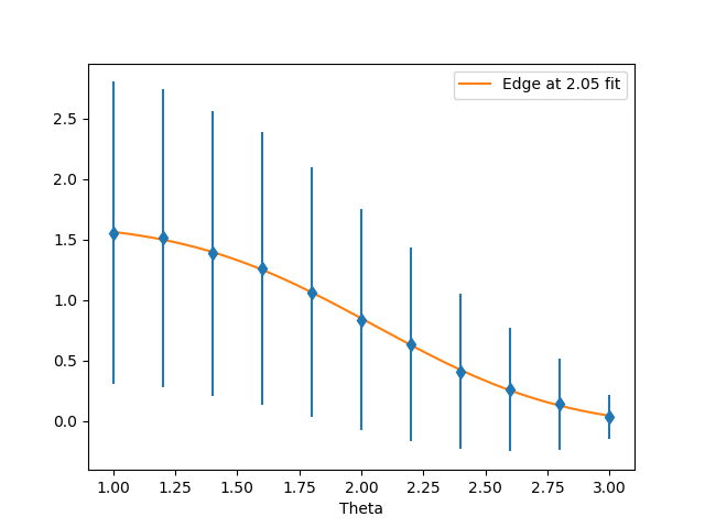

Similarly, there’s a top hat to simulate two edges

>>> fit = scan(theta, start=0, stop=2, count=11, fit=TopHat, frames=5, save="tophat.png")
Taking a count at theta=0.00 and two theta=0.00
Taking a count at theta=0.20 and two theta=0.00
Taking a count at theta=0.40 and two theta=0.00
Taking a count at theta=0.60 and two theta=0.00
Taking a count at theta=0.80 and two theta=0.00
Taking a count at theta=1.00 and two theta=0.00
Taking a count at theta=1.20 and two theta=0.00
Taking a count at theta=1.40 and two theta=0.00
Taking a count at theta=1.60 and two theta=0.00
Taking a count at theta=1.80 and two theta=0.00
Taking a count at theta=2.00 and two theta=0.00
>>> abs(fit["center"] - 1.0) < 0.1
True

If you need to do something really tricky, it’s possible to pull out the exact points.

>>> fit = scan(theta, start=0, stop=2, count=11, fit=ExactPoints, frames=5, save="exactpoints.png")
Taking a count at theta=0.00 and two theta=0.00
Taking a count at theta=0.20 and two theta=0.00
Taking a count at theta=0.40 and two theta=0.00
Taking a count at theta=0.60 and two theta=0.00
Taking a count at theta=0.80 and two theta=0.00
Taking a count at theta=1.00 and two theta=0.00
Taking a count at theta=1.20 and two theta=0.00
Taking a count at theta=1.40 and two theta=0.00
Taking a count at theta=1.60 and two theta=0.00
Taking a count at theta=1.80 and two theta=0.00
Taking a count at theta=2.00 and two theta=0.00
>>> fit["x"][-1]
2.0

Perform complex scans

Some uses need more complicated measurements that just a simple scan over a single axis. These more complicated commands may need some initial coaching from the beamline scientist, but should be simple enough for the user to modify them without assistance.

>>> th= scan(theta, start=0, stop=1, stride=0.3)

The above command does not contain a time command, so it does not run the full scan command. Instead, it merely creates a scan object, which is then stored in the th variable.

To start with, a user may want to scan theta and two theta together in lock step.

>>> two_th= scan(two_theta, start=0, stop=2, stride=0.6)
>>> (th& two_th).plot(frames=10, save="locked.png")
Taking a count at theta=0.00 and two theta=0.00
Taking a count at theta=0.25 and two theta=0.50
Taking a count at theta=0.50 and two theta=1.00
Taking a count at theta=0.75 and two theta=1.50
Taking a count at theta=1.00 and two theta=2.00

On the other hand, if the user is unsure about the proper sample alignment, they may want to investigate theta and two-theta separately

>>> th = scan(theta, start=0, stop=12, stride=0.5)
>>> two_th = scan(two_theta, start=0, stop=2, stride=0.5)
>>> (th * two_th).plot(frames=5, save="2d.png") # doctest: +ELLIPSIS
Taking a count at theta=0.00 and two theta=0.00
Taking a count at theta=0.00 and two theta=0.50
Taking a count at theta=0.00 and two theta=1.00
Taking a count at theta=0.00 and two theta=1.50
Taking a count at theta=0.00 and two theta=2.00
Taking a count at theta=0.50 and two theta=0.00
Taking a count at theta=0.50 and two theta=0.50
Taking a count at theta=0.50 and two theta=1.00
Taking a count at theta=0.50 and two theta=1.50
Taking a count at theta=0.50 and two theta=2.00
...
Taking a count at theta=11.50 and two theta=0.00
Taking a count at theta=11.50 and two theta=0.50
Taking a count at theta=11.50 and two theta=1.00
Taking a count at theta=11.50 and two theta=1.50
Taking a count at theta=11.50 and two theta=2.00
Taking a count at theta=12.00 and two theta=0.00
Taking a count at theta=12.00 and two theta=0.50
Taking a count at theta=12.00 and two theta=1.00
Taking a count at theta=12.00 and two theta=1.50
Taking a count at theta=12.00 and two theta=2.00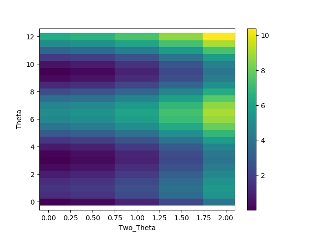

Two scans can also be run one after the other. If there are any overlapping points, then the measurement at that location will be performed twice and the results combined. This can allow for iterative scanning to improve statistics.

>>> two_theta(3.0)
>>> th = scan(theta, start=0, stop=1, stride=0.5)
>>> (th + th + th).plot(frames=5)
Taking a count at theta=0.00 and two theta=3.00
Taking a count at theta=0.50 and two theta=3.00
Taking a count at theta=1.00 and two theta=3.00
Taking a count at theta=0.00 and two theta=3.00
Taking a count at theta=0.50 and two theta=3.00
Taking a count at theta=1.00 and two theta=3.00
Taking a count at theta=0.00 and two theta=3.00
Taking a count at theta=0.50 and two theta=3.00
Taking a count at theta=1.00 and two theta=3.00

A scan can also be run in the reverse direction, if desired.

>>> th.reverse.plot(frames=5)
Taking a count at theta=1.00 and two theta=3.00
Taking a count at theta=0.50 and two theta=3.00
Taking a count at theta=0.00 and two theta=3.00

To minimise motor movement, a scan can turn around at its end and run backwards to collect more statistics

>>> th.and_back.plot(frames=5)
Taking a count at theta=0.00 and two theta=3.00
Taking a count at theta=0.50 and two theta=3.00
Taking a count at theta=1.00 and two theta=3.00
Taking a count at theta=1.00 and two theta=3.00
Taking a count at theta=0.50 and two theta=3.00
Taking a count at theta=0.00 and two theta=3.00

For a more interactive experience, a scan be set to cycle forever, improving the statistics until the use manually kills the scan.

>>> scan(theta, start=0, stop=1, stride=0.5).forever.fit(Gaussian, frames=5) #doctest: +SKIP

Estimate time

It’s not all that uncommon for users to find themselves setting an overnight run to perform while they sleep. Since they are usually writing these scripts around two in the morning, their arithemtic skills frequently fail. When the run terminates prematurely, the beam time is wasted. When the user underestimates the time that they’re requesting, they wake up to find that their measurements haven’t finished and they must use more beam time to finish their results.

Having the scan system perform estimates of the time required and the point of completion is a simple convenience to prevent these user headaches.

>>> scan(theta, start=0, stop=2.0, step=0.6).calculate(frames=50)
20.0
>>> scan(theta, start=0, stop=2.0, step=0.6).calculate(uamps=0.1)
36.0
>>> scan(theta, start=0, stop=2.0, step=0.6).calculate(hours=1.0)
14400.0
>>> scan(theta, start=0, stop=2.0, step=0.6).calculate(minutes=1.0)
240.0
>>> scan(theta, start=0, stop=2.0, step=0.6).calculate(seconds=5.0)
20.0

>>> needed = scan(theta, start=0, stop=2.0, step=0.6).calculate(frames=1000, time=True) #doctest: +SKIP
The run would finish at 2017-07-17 20:06:24.600802
>>> print(needed) #doctest: +SKIP
400.0

SPEC compatibility

As a convenience to users with an x-ray background, the ascan and dscan from SPEC have been implemented on top of the scanning interface. The only major change is that negative times now represent a number of frames instead of a monitor count, since waiting for a monitor count is currently unsupported.

>>> ascan(theta, 0, 2, 10, 1)
Taking a count at theta=0.00 and two theta=3.00
Taking a count at theta=0.20 and two theta=3.00
Taking a count at theta=0.40 and two theta=3.00
Taking a count at theta=0.60 and two theta=3.00
Taking a count at theta=0.80 and two theta=3.00
Taking a count at theta=1.00 and two theta=3.00
Taking a count at theta=1.20 and two theta=3.00
Taking a count at theta=1.40 and two theta=3.00
Taking a count at theta=1.60 and two theta=3.00
Taking a count at theta=1.80 and two theta=3.00
Taking a count at theta=2.00 and two theta=3.00
>>> theta(0.5)
>>> dscan(theta, -1, 1, 10, -50)
Traceback (most recent call last):
    ...
RuntimeError: Position -0.5 is below lower limit 0 of motor Theta
>>> theta(2.5)
>>> dscan(theta, -1, 1, 10, -50)
Taking a count at theta=1.50 and two theta=3.00
Taking a count at theta=1.70 and two theta=3.00
Taking a count at theta=1.90 and two theta=3.00
Taking a count at theta=2.10 and two theta=3.00
Taking a count at theta=2.30 and two theta=3.00
Taking a count at theta=2.50 and two theta=3.00
Taking a count at theta=2.70 and two theta=3.00
Taking a count at theta=2.90 and two theta=3.00
Taking a count at theta=3.10 and two theta=3.00
Taking a count at theta=3.30 and two theta=3.00
Taking a count at theta=3.50 and two theta=3.00
>>> theta
Theta is at 2.5

Position Commands

The user needs to give three of the following keyword arguments to create a scan.

start:This is the initial position of the scan. Fnord stop:This is the final position of the scan. The type of step chosen determines whether or not this final value is guaranteed to be included in the final measurement. before:This sets the initial position relative to the current position. after:This sets the final position relative to the current position. count:The total number of measurements to perform. This parameter always take precedence over “gaps” gaps:The number steps to take. The total number of measurements is always one greater than the number of gaps. stride:A requested, but not mandatory, step size. Users often know the range over which they wish to scan and their desired scanning resolution. stride measured the entire range, but may increase the resolution to give equally spaced measurements. stride always take precedence over step step:A mandatory step size. If the request measurement range is not an integer number of steps, the measurement will stop before the requested end.

See the Scans.Util.get_points() function for more information on the parameters.

Class setup

The base class for the low level code is the Scan class. This ensures that any functionality added to this class or bugs fixed in its code propagate out to all callers of this library. Unfortunately, Python does not have a concept of interfaces, so we cannot force all children to have a set of defined functions. However, any subclasses of Scan must contain the follow member functions:

map:Create a modified version of the scan based on a user supplied function. The original position of each point is fed as input to the function and the return value of the function is the new position. reverse:Create a copy of the scan that runs in the opposite direction. Reverse should be a property, since it takes no parameters __len__:Return the number of elements in the scan __iter__:Return an iterator that steps through the scan one position at a time, yielding the current position at each point.

There are four default subclasses of Scan that should handle most of the requirements

SimpleScan

is the lowest level of the scan system. It requires a function which performs the desired action on each point, a list of points, and a name for the axis. At this time, all scans are combinations of simpleScans.

SumScan

runs two scans sequentially. These scans do not need to be on the same axes or even move the same number of axes.

ProductScan

performs every possible combination of positions for two different scans. This provides an alternative to nested loops.

ParallelScan

takes to scans and runs their actions together at each step. For example, if a' was a scan over theta and `b was a scan over two theta, then a && b would scan each theta angle with its corresponding two theta.

The base Scan class contains four useful member functions.

plot:The plot function goes to each position listed in the scan, takes a count, and plots it on an axis. The user can specify the counting command. measure:The measure function goes to each position in the in the scan and records a measurement. The function is passed a title which can include information about the current position in the scan. fit:Like plot, this function takes a single count at each position. It then fits it to the user supplied model and returns the fitted value. This could be anything from the peak position to the frequency of the curve. calculate:This function takes a desired measurement time at each point and, optionally, an approximated motor movement time. It returns an estimated duration for the scan and time of completion.

Design Goals

This is a proposal for an improved system for running scans on the instrument. The idea is to use Scan objects to represent the parts of the scan. These scan objects form an algebra, making them easier to compose than using for loops. These scan objects are mainly intended as tools for the instrument scientists for creating a higher level interface that the users will interact with.

We desire the following traits in the Scanning system

User simplicity

The users need to be able to perform simple scans without thinking about object orient programming or algebraic data types. Performing a basic scan should always be a one liner. Making modified versions of that scan should require learning a modification of that command and not an entirely new structure. Common, sensible user options should be available and sane defaults given.

The code should also take advantage of Python’s built in documentation system to allow for discoverability of all of the functionality of these scripts.

Composability

The code should trivially allow combining smaller scripts into a larger script. This ensures that, as long as the smaller scripts are bug free, the larger scripts will also be free of bugs by construction.

Functionality

The code should be able to perform all of the tasks that might involve scanning on the beamline, from the common place to the irregular.

Plotting: It should be possible to plot any readback value as a function

of any set of motor positions. Scans of multiple axes should be able to either plot multiple labelled lines or a 2D heatmap

Measuring: Performing a full series of measurements should only be a

minor modification of the plotting command

Fitting: The user should be capable of performing fits on curves to

extract values of interest. Common fitting routines should be a simple string while still accepting custom functions for exceptional circumstances

Spacing: It should be possible to space points both linearly and

logarithmically.

Prediction: It should be possible to estimate the time needed for a scan

before the scan is performed.